Edges

Edge Detection

Edges are local features that capture important information of the semantic content of the image. They are defined as the set of pixels laying between two image regions with different light intensity

1 dimensional step edge

In this situation an edge can be seen as a peak of the first derivative of the intensity pixel function

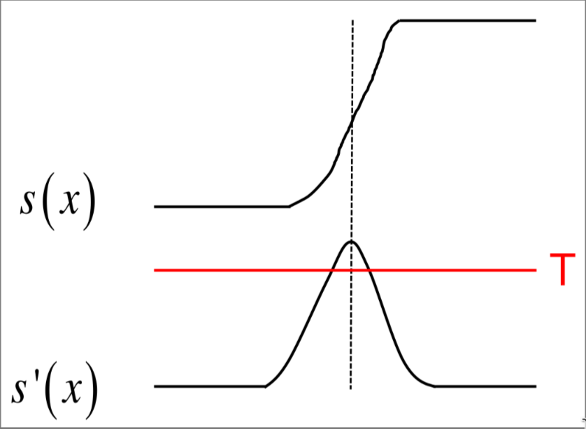
So in order to detect edge in this situation is sufficient to threshold the first derivative

flowchart LR A["S(x)"] B["d(S)"] C[T] D["e(x)"] A --> B --> C --> D

2 dimensional step edge

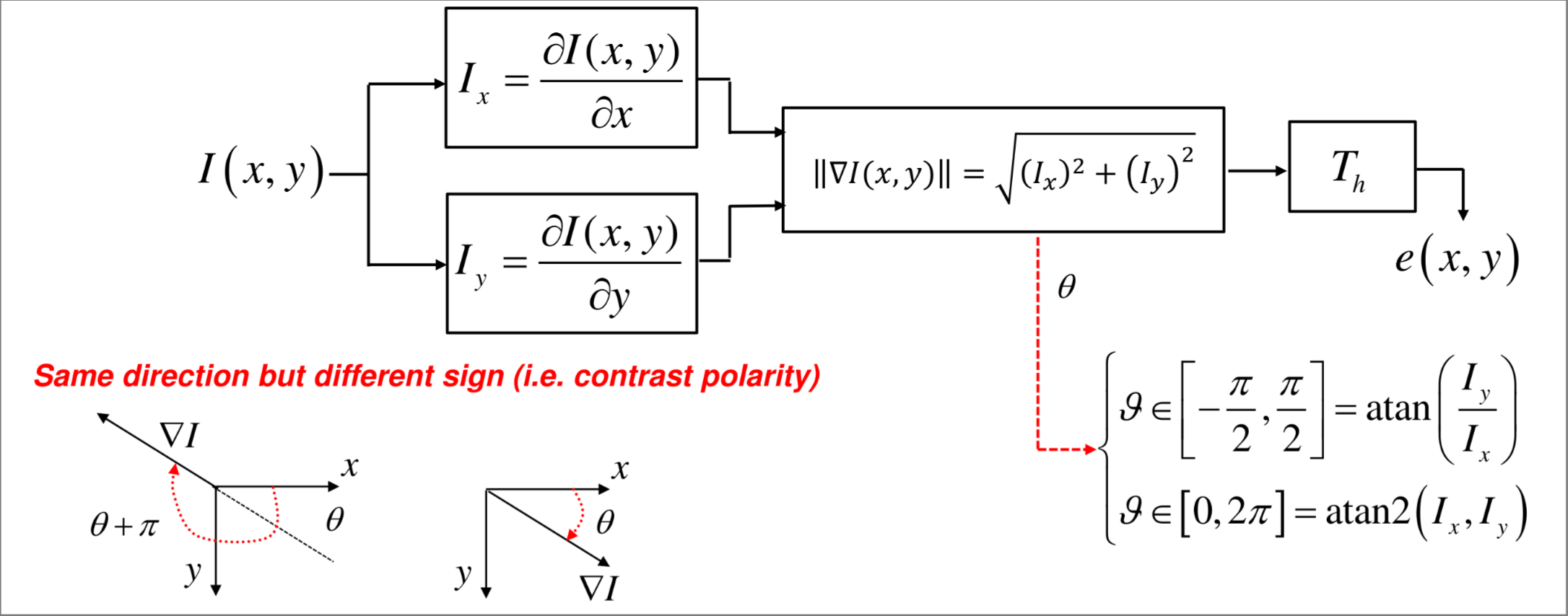
In a 2D image input signal edge is characterized also by direction, In this context the derivative is no more sufficient and the gradient function is used

$$ \nabla I(x,y) = \frac{\delta I(x,y)}{\delta x}i +\frac{\delta I(x,y)}{\delta y}j $$ The gradient direction is the direction where the intensity function show the maximum variation

First detection pipeline

Gradient approximation

In order to compute the gradient efficiently a discrete approximation is needed, multiple choices are possible

backward or forward differences

$$ \frac{\delta I(x,y)}{\delta x} \simeq = I(i,j) - I(i,j-1) $$ $$ \frac{\delta I(x,y)}{\delta x} \simeq = I(i,j+1) - I(i,j) $$

$$ \frac{\delta I(x,y)}{\delta y} \simeq = I(i,j) - I(i -1,j) $$ $$ \frac{\delta I(x,y)}{\delta y} \simeq = I(i+1,j) - I(i,j) $$

or central differences

$$ \frac{\delta I(x,y)}{\delta y} \simeq = I(i,j + 1) - I(i,j-1) $$ $$ \frac{\delta I(x,y)}{\delta y} \simeq = I(i+1,j) - I(i-1,j) $$

There are also a lot of ways to approximate the gradient intensity

$$ \Vert \nabla I\Vert_2 = \sqrt{I_x^2 + I_y^2} \space $$ $$ \Vert \nabla I\Vert_1 = \vert I_x + I_y \vert \space $$ $$ \Vert \nabla I\Vert_{\infty} = \max{(I_x , I_y)} \space $$

Noise problems

Due to the nature of the derivative operation of amplifying noise the input signal needs to be smoothed out to allow a correct edge detection

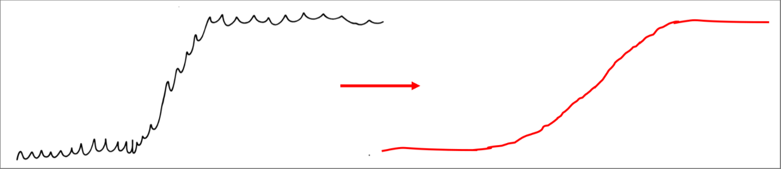
the smoothing process and the derivative can be carried out by a single operation using the mean of point in the derivative approximation step

$$ \mu_x = \frac{1}{3}(I(i,j-1),I(i,j),I(i,j+1)) \ $$ $$ \mu_y = \frac{1}{3}(I(i-1,j),I(i,j),I(i+1,j)) \ $$

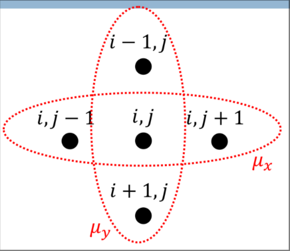
And then the derivative is obtained by the difference of the means

$$ \overset{\sim}I_x = \mu_x(i,j+1) - \mu_x(i,j) $$ $$ \overset{\sim}I_y = \mu_x(i+1,j) - \mu_x(i,j) $$

Derivative variants

There are some operator with some additional features

Prewitt operator which takes into account central differences (better for diagonal edges) $$ \overset{\sim}I_x(i,j) = \mu_x(i+1,j)+\mu_x(i-1,j) $$ $$ \overset{\sim}I_y(i,j) = \mu_y(i+1,j)+\mu_y(i-1,j) $$
Sobel operator which Weights more the point on the center in order to improve isotropy $$ \overset{\sim}I_x(i,j) = \mu_x(i+1,j)+\mu_x(i-1,j) $$ $$ \mu_x(i,j) = \frac{1}{k+2}[I(i+1,j)+kI(i-1,j)+I(i-1,j)] $$

Finding maxima to localize edges

It’s difficult to localize edge in an image just by thresholding, a too low threshold could result in a poor localization of the edge (e.g. thick edges)

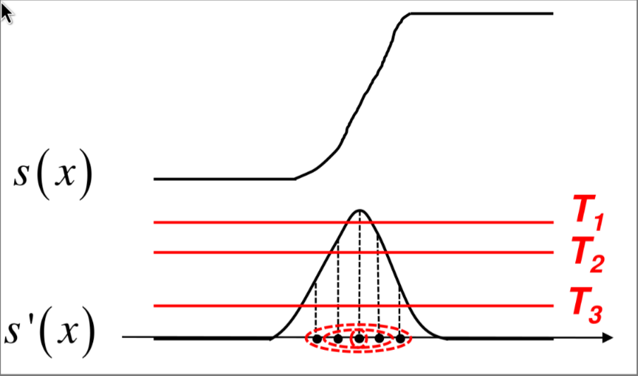
A better way to localize the edges is to find the local maxima of the absolute value of the derivative

Non maxima supression (nms)

The idea is to use the discrete representation of the gradient discussed earlier to compute an algorithm that identifies local maxima points.

So given a point in an image

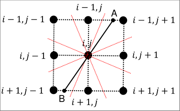
The gradient in the line from $A$ to $B$ can be approximated as follows

$$ G = \Vert \nabla I(i,j)\Vert $$ $$ G_A \simeq \Vert \nabla I(i-1,j+1)\Vert $$ $$ G_B \simeq \Vert \nabla I(i+1,j-1)\Vert $$

And with this approximation the NMS can be obtained as follows

$$ NMS(i,j) = \begin{cases} 1 : (G \gt G_A )\land (G \gt G_B) \ 0: otherwise \end{cases} $$

Final edge detector pipeline

With this considerations the final edge detection pipeline looks like this

flowchart LR A["I"] B["I_x"] C["I_y"] D["|| I ||"] E["NMS"] F["T_h"] G["E"] A --> B & C --> D --> E --> F --> G

There is a final thresholding step in order to avoid detection of unwanted edges.

previous next